6. Land Data Assimilation System

This chapter describes the configuration of the offline Land Data Assimilation (DA) System, which utilizes the UFS Noah-MP components with the JEDI fv3-bundle to enable cycled model forecasts. The data assimilation framework applies the Local Ensemble Transform Kalman Filter-Optimal Interpolation (LETKF-OI) algorithm to combine the state-dependent background error derived from an ensemble forecast with the observations and their corresponding uncertainties to produce an analysis ensemble (Hunt et al. [HEJKS07], 2007).

6.1. Joint Effort for Data Assimilation Integration (JEDI)

The Joint Effort for Data assimilation Integration (JEDI) is a unified and versatile data assimilation (DA) system for Earth System Prediction that can be run on a variety of platforms. JEDI is developed by the Joint Center for Satellite Data Assimilation (JCSDA) and partner agencies, including NOAA. The core feature of JEDI is separation of concerns. The data assimilation update, observation selection and processing, and observation operators are all coded with no knowledge of or dependency on each other or on the forecast model.

The NOAH-MP offline Land DA System uses three JEDI components:

• The Object-Oriented Prediction System (OOPS) for the data assimilation algorithm

• The Interface for Observation Data Access (IODA) for the observation formatting and processing

• The Unified Forward Operator (UFO) for comparing model forecasts and observations

JEDI’s Unified Forward Operator (UFO) links observation operators with the Object Oriented Prediction System (OOPS) to compute a simulated observation given a known model state. It does not restrict observation operators based on model-specific code structures or requirements. The UFO code structure provides generic classes for observation bias correction and quality control. Within this system, IODA converts the observation data into model-specific formats to be ingested by each model’s data assimilation system. This involves model-specific data conversion efforts.

6.1.1. Object-Oriented Prediction System (OOPS)

A data assimilation experiment requires a yaml configuration file that specifies the details of the data assimilation and observation processing. OOPS provides the core set of data assimilation algorithms in JEDI by combining the generic building blocks required for the algorithms. The OOPS system does not require knowledge of any specific application model implementation structure or observation data information. In the Noah-MP offline Land DA System, OOPS reads the model forecast states from the restart files generated by the Noah-MP model. JEDI UFO contains generic quality control options and filters that can be applied to each observation system, without coding at certain model application levels. More information on the key concepts of the JEDI software design can be found in Trémolet and Auligné [TA20] (2020), Holdaway et al. [HVMWK20] (2020), and Honeyager et al. [HHZ+20] (2020).

6.1.1.1. JEDI Configuration Files & Parameters

To create the DA experiment, the user should create or modify an experiment-specific configuration yaml file. This yaml file should contain certain fundamental components: geometry, window begin, window length, background, driver, local ensemble DA, output increment, and observations. These components can be implemented differently for different models and observation types, so they frequently contain distinct parameters and variable names depending on the use case. Therefore, this section of the User’s Guide focuses on assisting users with understanding and customizing these top-level configuration items in order to run Land DA experiments. Users may also reference the JEDI Documentation for additional information.

Users may find the following example yaml configuration file to be a helpful starting point. This file (with user-appropriate modifications) is required by JEDI for snow data assimilation. The following subsections will explain the variables within each top-level item of the yaml file.

geometry:
  fms initialization:
    namelist filename: Data/fv3files/fmsmpp.nml
    field table filename: Data/fv3files/field_table
  akbk: Data/fv3files/akbk127.nc4
  npx: 97
  npy: 97
  npz: 127
  field metadata override: Data/fieldmetadata/gfs-land.yaml
  time invariant fields:
    state fields:
      datetime: 2016-01-02T18:00:00Z
      filetype: fms restart
      skip coupler file: true
      state variables: [orog_filt]
      datapath: /mnt/lfs4/HFIP/hfv3gfs/role.epic/landda/inputs/forcing/gdas/orog_files
      filename_orog: oro_C96.mx100.nc

window begin: 2016-01-02T12:00:00Z
window length: PT6H

background:
  date: &date 2016-01-02T18:00:00Z
  members:
    - datetime: 2016-01-02T18:00:00Z
      filetype: fms restart
      state variables: [snwdph,vtype,slmsk]
      datapath: mem_pos/
      filename_sfcd: 20160102.180000.sfc_data.nc
      filename_cplr: 20160102.180000.coupler.res
    - datetime: 2016-01-02T18:00:00Z
      filetype: fms restart
      state variables: [snwdph,vtype,slmsk]
      datapath: mem_neg/
      filename_sfcd: 20160102.180000.sfc_data.nc
      filename_cplr: 20160102.180000.coupler.res

driver:
  save posterior mean: false
  save posterior mean increment: true
  save posterior ensemble: false
  run as observer only: false

local ensemble DA:
  solver: LETKF
  inflation:
    rtps: 0.0
    rtpp: 0.0
    mult: 1.0

output increment:
  filetype: fms restart
  filename_sfcd: xainc.sfc_data.nc

observations:
  observers:
  - obs space:
      name: Simulate
      distribution:
        name: Halo
        halo size: 250e3
      simulated variables: [totalSnowDepth]
      obsdatain:
        engine:
          type: H5File
          obsfile: GHCN_2016010218.nc
      obsdataout:
        engine:
          type: H5File
          obsfile: output/DA/hofx/letkf_hofx_ghcn_2016010218.nc
    obs operator:
      name: Identity
    obs error:
      covariance model: diagonal
    obs localizations:
    - localization method: Horizontal SOAR
      lengthscale: 250e3
      soar horizontal decay: 0.000021
      max nobs: 50
    - localization method: Vertical Brasnett
      vertical lengthscale: 700
    obs filters:
    - filter: Bounds Check # negative / missing snow
      filter variables:
      - name: totalSnowDepth
      minvalue: 0.0
    - filter: Domain Check # missing station elevation (-999.9)
      where:
      - variable:
          name: height@MetaData
        minvalue: -999.0
    - filter: Domain Check # land only
      where:
      - variable:
          name: slmsk@GeoVaLs
        minvalue: 0.5
        maxvalue: 1.5
    # GFSv17 only.
    #- filter: Domain Check # no sea ice
    #  where:
    #  - variable:
    #      name: fraction_of_ice@GeoVaLs
    #    maxvalue: 0.0
    - filter: RejectList  # no land-ice
      where:
      - variable:
          name: vtype@GeoVaLs
        minvalue: 14.5
        maxvalue: 15.5
    - filter: Background Check # gross error check
      filter variables:
      - name: totalSnowDepth
      threshold: 6.25
      action:
        name: reject

Note

Any default values indicated in the sections below are the defaults set in letkfoi_snow.yaml or GHCN.yaml (found within the land-offline_workflow/DA_update/jedi/fv3-jedi/yaml_files/release-v1.0/ directory).

6.1.1.1.1. Geometry

The geometry: section is used in JEDI configuration files to specify the model grid’s parallelization across compute nodes (horizontal and vertical).

fms initialization

This section contains two parameters, namelist filename and field table filename.

namelist filename

Specifies the path for the namelist filename.

field table filename

Specifies the path for the field table filename.

akbk

Specifies the path to a file containing the coefficients that define the hybrid sigma-pressure vertical coordinate used in FV3. Files are provided with the repository containing ak and bk for some common choices of vertical resolution for GEOS and GFS.

npx

Specifies the number of grid cells in the east-west direction.

npy

Specifies the number of grid cells in the north-south direction.

npz

Specifies the number of vertical layers.

field metadata override

Specifies the path for file metadata.

time invariant state fields

This parameter contains several subparameters listed below.

datetime

Specifies the time in YYYY-MM-DDTHH:00:00Z format, where YYYY is a 4-digit year, MM is a valid 2-digit month, DD is a valid 2-digit day, and HH is a valid 2-digit hour.

filetype

Specifies the type of file. Valid values include: fms restart

skip coupler file

Specifies whether to enable skipping coupler file. Valid values are: true | false

Value	Description
true	enable
false	do not enable

state variables

Specifies the list of state variables. Valid values include: [orog_filt]

datapath

Specifies the path for state variables data.

filename_orog

Specifies the name of orographic data file.

6.1.1.1.2. Window begin, Window length

These two items define the assimilation window for many applications, including Land DA.

window begin:

Specifies the beginning time window. The format is YYYY-MM-DDTHH:00:00Z, where YYYY is a 4-digit year, MM is a valid 2-digit month, DD is a valid 2-digit day, and HH is a valid 2-digit hour.

window length:

Specifies the time window length. The form is PTXXH, where XX is a 1- or 2-digit hour. For example: PT6H

6.1.1.1.3. Background

The background: section includes information on the analysis file(s) (also known as “members”) generated by the previous cycle.

date

Specifies the background date. The format is &date YYYY-MM-DDTHH:00:00Z, where YYYY is a 4-digit year, MM is a valid 2-digit month, DD is a valid 2-digit day, and HH is a valid 2-digit hour. For example: &date 2016-01-02T18:00:00Z

members

Specifies information on analysis file(s) generated by a previous cycle.

datetime

Specifies the date and time. The format is YYYY-MM-DDTHH:00:00Z, where YYYY is a 4-digit year, MM is a valid 2-digit month, DD is a valid 2-digit day, and HH is a valid 2-digit hour.

filetype

Specifies the type of file. Valid values include: fms restart

state variables

Specifies a list of state variables. Valid values: [snwdph,vtype,slmsk]

datapath

Specifies the path for state variables data. Valid values: mem_pos/ | mem_neg/. (With default experiment values, the full path will be workdir/mem000/jedi/$datapath.)

filename_sfcd

Specifies the name of the surface data file. This usually takes the form YYYYMMDD.HHmmss.sfc_data.nc, where YYYY is a 4-digit year, MM is a valid 2-digit month, DD is a valid 2-digit day, and HH is a valid 2-digit hour, mm is a valid 2-digit minute and ss is a valid 2-digit second. For example: 20160102.180000.sfc_data.nc

filename_cprl

Specifies the name of file that contains metadata for the restart. This usually takes the form YYYYMMDD.HHmmss.coupler.res, where YYYY is a 4-digit year, MM is a valid 2-digit month, DD is a valid 2-digit day, and HH is a valid 2-digit hour, mm is a valid 2-digit minute and ss is a valid 2-digit second. For example: 20160102.180000.coupler.res

6.1.1.1.4. Driver

The driver: section describes optional modifications to the behavior of the LocalEnsembleDA driver. For details, refer to Local Ensemble Data Assimilation in OOPS in the JEDI Documentation.

save posterior mean

Specifies whether to save the posterior mean. Valid values: true | false

Value	Description
true	save
false	do not save

save posterior mean increment

Specifies whether to save the posterior mean increment. Valid values: true | false

Value	Description
true	enable
false	do not enable

save posterior ensemble

Specifies whether to save the posterior ensemble. Valid values: true | false

Value	Description
true	enable
false	do not enable

run as observer only

Specifies whether to run as observer only. Valid values: true | false

Value	Description
true	enable
false	do not enable

6.1.1.1.5. Local Ensemble DA

The local ensemble DA: section configures the local ensemble DA solver package.

solver

Specifies the type of solver. Currently, LETKF is the only available option. See Hunt et al. [HEJKS07] (2007).

inflation

Describes ensemble inflation methods.

rtps: (Default: 0.0)

Relaxation to prior spread (Whitaker and Hamill [WH12], 2012).

rtpp: (Default: 0.0)

Relaxation to prior perturbation (Zhang et al. [ZCSS04], 2004).

mult: (Default: 1.0)

Parameter of multiplicative inflation.

6.1.1.1.6. Output Increment

output increment:

filetype

Type of file provided for the output increment. Valid values include: fms restart

filename_sfcd

Name of the file provided for the output increment. For example: xainc.sfc_data.nc

6.1.1.1.7. Observations

The observations: item describes one or more types of observations, each of which is a multi-level YAML/JSON object in and of itself. Each of these observation types is read into JEDI as an eckit::Configuration object (see JEDI Documentation for more details).

6.1.1.1.7.1. obs space:

The obs space: section of the yaml comes under the observations.observers: section and describes the configuration of the observation space. An observation space handles observation data for a single observation type.

name

Specifies the name of observation space. The Land DA System uses Simulate for the default case.

distribution:

name

Specifies the name of distribution. Valid values include: Halo

halo size

Specifies the size of the halo distribution. Format is e-notation. For example: 250e3

simulated variables

Specifies the list of variables that need to be simulated by observation operator. Valid values: [totalSnowDepth]

obsdatain

This section specifies information about the observation input data.

engine

This section specifies parameters required for the file matching engine.

type

Specifies the type of input observation data. Valid values: H5File | OBS

obsfile

Specifies the input filename.

obsdataout

This section contains information about the observation output data.

engine

This section specifies parameters required for the file matching engine.

type

Specifies the type of output observation data. Valid values: H5File

obsfile

Specifies the output file path.

6.1.1.1.7.2. obs operator:

The obs operator: section describes the observation operator and its options. An observation operator is used for computing H(x).

name

Specifies the name in the ObsOperator and LinearObsOperator factory, defined in the C++ code. Valid values include: Identity. See JEDI Documentation for more options.

6.1.1.1.7.3. obs error:

The obs error: section explains how to calculate the observation error covariance matrix and gives instructions (required for DA applications). The key covariance model, which describes how observation error covariances are created, is frequently the first item in this section. For diagonal observation error covariances, only the diagonal option is currently supported.

covariance model

Specifies the covariance model. Valid values include: diagonal

6.1.1.1.7.4. obs localizations:

obs localizations:

localization method

Specifies the observation localization method. Valid values include: Horizontal SOAR

Value	Description
Horizontal SOAR	Second Order Auto-Regressive localization in the horizontal direction.
Vertical Brasnett	Vertical component of the localization scheme defined in Brasnett [Bra99] (1999) and used in the snow DA.

lengthscale

Radius of influence (i.e., maximum distance of observations from the location being updated) in meters. Format is e-notation. For example: 250e3

soar horizontal decay

Decay scale of SOAR localization function. Recommended value: 0.000021. Users may adjust based on need/preference.

max nobs

Maximum number of observations used to update each location.

6.1.1.1.7.5. obs filters:

Observation filters are used to define Quality Control (QC) filters. They have access to observation values and metadata, model values at observation locations, simulated observation value, and their own private data. See Observation Filters in the JEDI Documentation for more detail. The obs filters: section contains the following fields:

filter

Describes the parameters of a given QC filter. Valid values include: Bounds Check | Background Check | Domain Check | RejectList. See descriptions in the JEDI’s Generic QC Filters Documentation for more.

Filter Name	Description
Bounds Check	Rejects observations whose values lie outside specified limits:
Background Check	This filter checks for bias-corrected distance between the observation value and model-simulated value (y - H(x)) and rejects observations where the absolute difference is larger than the absolute threshold or threshold * observation error or threshold * background error.
Domain Check	This filter retains all observations selected by the where statement and rejects all others.
RejectList	This is an alternative name for the BlackList filter, which rejects all observations selected by the where statement. The status of all others remains the same. Opposite of Domain Check filter.

filter variables

Limit the action of a QC filter to a subset of variables or to specific channels.

name

Name of the filter variable. Users may indicate additional filter variables using the name field on consecutive lines (see code snippet below). Valid values include: totalSnowDepth

filter variables:
- name: variable_1
- name: variable_2

minvalue

Minimum value for variables in the filter.

maxvalue

Maximum value for variables in the filter.

threshold

This variable may function differently depending on the filter it is used in. In the Background Check Filter, an observation is rejected when the difference between the observation value (y) and model simulated value (H(x)) is larger than the threshold * observation error.

action

Indicates which action to take once an observation has been flagged by a filter. See Filter Actions in the JEDI documentation for a full explanation and list of valid values.

name

The name of the desired action. Valid values include: accept | reject

where

By default, filters are applied to all filter variables listed. The where keyword applies a filter only to observations meeting certain conditions. See the Where Statement section of the JEDI Documentation for a complete description of valid where conditions.

variable

A list of variables to check using the where statement.

name

Name of a variable to check using the where statement. Multiple variable names may be listed under variable. The conditions in the where statement will be applied to all of them. For example:

filter: Domain Check # land only
  where:
  - variable:
      name: variable_1
      name: variable_2
    minvalue: 0.5
    maxvalue: 1.5

minvalue

Minimum value for variables in the where statement.

maxvalue

Maximum value for variables in the where statement.

6.1.2. Interface for Observation Data Access (IODA)

This section references Honeyager, R., Herbener, S., Zhang, X., Shlyaeva, A., and Trémolet, Y., 2020: Observations in the Joint Effort for Data assimilation Integration (JEDI) - UFO and IODA. JCSDA Quarterly, 66, Winter 2020.

The Interface for Observation Data Access (IODA) is a subsystem of JEDI that can handle data processing for various models, including the Land DA System. Currently, observation data sets come in a variety of formats (e.g., netCDF, BUFR, GRIB) and may differ significantly in structure, quality, and spatiotemporal resolution/density. Such data must be pre-processed and converted into model-specific formats. This process often involves iterative, model-specific data conversion efforts and numerous cumbersome ad-hoc approaches to prepare observations. Requirements for observation files and I/O handling often result in decreased I/O and computational efficiency. IODA addresses this need to modernize observation data management and use in conjunction with the various components of the Unified Forecast System (UFS).

IODA provides a unified, model-agnostic method of sharing observation data and exchanging modeling and data assimilation results. The IODA effort centers on three core facets: (i) in-memory data access, (ii) definition of the IODA file format, and (iii) data store creation for long-term storage of observation data and diagnostics. The combination of these foci enables optimal isolation of the scientific code from the underlying data structures and data processing software while simultaneously promoting efficient I/O during the forecasting/DA process by providing a common file format and structured data storage.

The IODA file format represents observational field variables (e.g., temperature, salinity, humidity) and locations in two-dimensional tables, where the variables are represented by columns and the locations by rows. Metadata tables are associated with each axis of these data tables, and the location metadata hold the values describing each location (e.g., latitude, longitude). Actual data values are contained in a third dimension of the IODA data table; for instance: observation values, observation error, quality control flags, and simulated observation (H(x)) values.

Since the raw observational data come in various formats, a diverse set of “IODA converters” exists to transform the raw observation data files into IODA format. While many of these Python-based IODA converters have been developed to handle marine-based observations, users can utilize the “IODA converter engine” components to develop and implement their own IODA converters to prepare arbitrary observation types for data assimilation within JEDI. (See https://github.com/NOAA-PSL/land-DA_update/blob/develop/jedi/ioda/imsfv3_scf2ioda_obs40.py for the land DA IMS IODA converter.)

6.2. Input Files

The Land DA System requires grid description files, observation files, and restart files to perform snow DA.

6.2.1. Grid Description Files

The grid description files appear in Section 5.2.1 and are also used as input files to the Vector-to-Tile Converter. See Table 5.3 for a description of these files.

6.2.2. Observation Data

Observation data from 2016 and 2020 are provided in NetCDF format for the v1.0.0 release. Instructions for downloading the data are provided in Section 4.3, and instructions for accessing the data on Level 1 Systems are provided in Section 3.2. Currently, data is taken from the Global Historical Climatology Network (GHCN), but eventually, data from the U.S. National Ice Center (USNIC) Interactive Multisensor Snow and Ice Mapping System (IMS) will also be available for use.

6.2.2.1. Observation Types

6.2.2.1.1. GHCN Snow Depth Files

Snow depth observations are taken from the Global Historical Climatology Network, which provides daily climate summaries sourced from a global network of 100,000 stations. NOAA’s NCEI provides access to these snow depth and snowfall measurements through daily-generated individual station ASCII files or GZipped tar files of full-network observations on the NCEI server or Climate Data Online. Alternatively, users may acquire yearly tarballs via wget:

wget https://www1.ncdc.noaa.gov/pub/data/ghcn/daily/by_year/{YYYY}.csv.gz

where ${YYYY} should be replaced with the year of interest. Note that these yearly tarballs contain all measurement types from the daily GHCN output, and thus, snow depth must be manually extracted from this broader data set.

These raw snow depth observations need to be converted into IODA-formatted netCDF files for ingestion into the JEDI LETKF system. However, this process was preemptively handled outside of the Land DA workflow, and the initial GHCN IODA files for 2016 and 2020 were provided by NOAA PSL (Clara Draper).

The IODA-formatted GHCN files are structured as follows (using 20160102 as an example):

netcdf ghcn_snwd_ioda_20160102 {
dimensions:
   nlocs = UNLIMITED ; // (9946 currently)
variables:
   int nlocs(nlocs) ;
                nlocs:suggested_chunk_dim = 9946LL ;

// global attributes:
      string :_ioda_layout = "ObsGroup" ;
      :_ioda_layout_version = 0 ;
      string :converter = "ghcn_snod2ioda_newV2.py" ;
      string :date_time_string = "2016-01-02T18:00:00Z" ;
      :nlocs = 9946 ;

group: MetaData {
   variables:
      string datetime(nlocs) ;
         string datetime:_FillValue = "" ;
      float height(nlocs) ;
         height:_FillValue = 9.96921e+36f ;
         string height:units = "m" ;
      float latitude(nlocs) ;
         latitude:_FillValue = 9.96921e+36f ;
         string latitude:units = "degrees_north" ;
      float longitude(nlocs) ;
         longitude:_FillValue = 9.96921e+36f ;
         string longitude:units = "degrees_east" ;
      string stationIdentification(nlocs) ;
         string stationIdentification:_FillValue = "" ;
   } // group MetaData

group: ObsError {
   variables:
      float totalSnowDepth(nlocs) ;
         totalSnowDepth:_FillValue = 9.96921e+36f ;
         string totalSnowDepth:coordinates = "longitude latitude" ;
         string totalSnowDepth:units = "mm" ;
   } // group ObsError

group: ObsValue {
   variables:
      float totalSnowDepth(nlocs) ;
         totalSnowDepth:_FillValue = 9.96921e+36f ;
         string totalSnowDepth:coordinates = "longitude latitude" ;
         string totalSnowDepth:units = "mm" ;
   } // group ObsValue

group: PreQC {
   variables:
      int totalSnowDepth(nlocs) ;
         totalSnowDepth:_FillValue = -2147483647 ;
         string totalSnowDepth:coordinates = "longitude latitude" ;
   } // group PreQC
}

The primary observation variable is totalSnowDepth, which, along with the metadata fields of datetime, latitude, longitude, and height is defined along the nlocs dimension. Also present are ObsError and PreQC values corresponding to each totalSnowDepth measurement on nlocs. These values were attributed during the IODA conversion step (not supported for this release). The magnitude of nlocs varies between files; this is due to the fact that the number of stations reporting snow depth observations for a given day can vary in the GHCN.

6.2.2.2. Observation Location and Processing

6.2.2.2.1. GHCN

GHCN files for 2016 and 2020 are already provided in IODA format for the v1.0.0 release. Table 3.2 indicates where users can find data on NOAA RDHPCS platforms. Tar files containing the 2016 and 2020 data are located in the publicly-available Land DA Data Bucket. Once untarred, the snow depth files are located in /inputs/DA/snow_depth/GHCN/data_proc/{YEAR}. These GHCN IODA files were provided by Clara Draper (NOAA PSL). Each file follows the naming convention of ghcn_snwd_ioda_${YYYY}${MM}${DD}.nc, where ${YYYY} is the four-digit cycle year, ${MM} is the two-digit cycle month, and ${DD} is the two-digit cycle day.

In each experiment, the DA_config file sets the name of the experiment configuration file. This configuration file is typically named settings_DA_test. Before assimilation, if “GHCN” was specified as the observation type in the DA_config file, the ghcn_snwd_ioda_${YYYY}${MM}${DD}.nc file corresponding to the specified cycle date is soft-linked to the JEDI working directory (${JEDIWORKDIR}) with a naming-convention change (i.e., GHCN_${YYYY}${MM}${DD}${HH}.nc). Here, the GHCN IODA file is appended with the cycle hour, ${HH} which is extracted from the ${STARTDATE} variable defined in the relevant DA_config file.

Prior to ingesting the GHCN IODA files via the LETKF at the DA analysis time, the observations are further quality controlled and checked using letkf_land.yaml (itself a concatenation of GHCN.yaml and letkfoi_snow.yaml; see the GitHub yaml files for more detail). The GHCN-specific observation filters, domain checks, and quality control parameters from GHCN.yaml ensure that only snow depth observations which meet specific criteria are assimilated (the rest are rejected). The contents of this YAML are listed below:

- obs space:
    name: Simulate
    distribution:
      name: Halo
      halo size: 250e3
    simulated variables: [totalSnowDepth]
    obsdatain:
      engine:
        type: H5File
        obsfile: GHCN_XXYYYYXXMMXXDDXXHH.nc
    obsdataout:
      engine:
        type: H5File
        obsfile: output/DA/hofx/letkf_hofx_ghcn_XXYYYYXXMMXXDDXXHH.nc
  obs operator:
    name: Identity
  obs error:
    covariance model: diagonal
  obs localizations:
  - localization method: Horizontal SOAR
    lengthscale: 250e3
    soar horizontal decay: 0.000021
    max nobs: 50
  - localization method: Vertical Brasnett
    vertical lengthscale: 700
  obs filters:
  - filter: Bounds Check # negative / missing snow
    filter variables:
    - name: totalSnowDepth
    minvalue: 0.0
  - filter: Domain Check # missing station elevation (-999.9)
    where:
    - variable:
        name: height@MetaData
      minvalue: -999.0
  - filter: Domain Check # land only
    where:
    - variable:
        name: slmsk@GeoVaLs
      minvalue: 0.5
      maxvalue: 1.5
  # GFSv17 only.
  #- filter: Domain Check # no sea ice
  #  where:
  #  - variable:
  #      name: fraction_of_ice@GeoVaLs
  #    maxvalue: 0.0
  - filter: RejectList  # no land-ice
    where:
    - variable:
        name: vtype@GeoVaLs
      minvalue: 14.5
      maxvalue: 15.5
  - filter: Background Check # gross error check
    filter variables:
    - name: totalSnowDepth
    threshold: 6.25
    action:
      name: reject

6.2.2.3. Viewing NetCDF Files

Users can view file information and notes for NetCDF files using the ncdump module. First, load a compiler, MPI, and NetCDF modules:

# To see available modules:
module avail
# To load modules:
module load intel/2022.2.0 impi/2022.2.0 netcdf/4.7.0

Users may need to modify the module load command to reflect modules that are available on their system.

Then, run ncdump -h path/to/file. For example, on Hera, users can run:

ncdump -h /scratch1/NCEPDEV/nems/role.epic/landda/inputs/DA/snow_depth/GHCN/data_proc/2016/ghcn_snwd_ioda_20160102.nc

to see the contents of the 2016-01-02 GHCN file.

6.2.3. Restart Files

To restart the ufs-land-driver successfully after land model execution, all parameters, states, and fluxes used for a subsequent time iteration are stored in a restart file. This restart file is named ufs_land_restart.{FILEDATE}.nc where FILEDATE is in YYYY-MM-DD_HH-mm-SS format (e.g., ufs_land_restart.2016-01-02_18-00-00.nc). The restart file contains all the model fields and their values at a specific point in time; this information can be used to restart the model immediately to run the next cycle. The Land DA System reads the states from the restart file and replaces them after the DA step with the updated analysis. Table 6.1 lists the fields in the Land DA restart file. Within the ufs-land-driver, read/write of the restart file is performed in ufsLandNoahMPRestartModule.f90.

Table 6.1 Files Included in ufs_land_restart.{FILEDATE}.nc

Variable	Long name	Unit
time	time	“seconds since 1970-01-01 00:00:00”
timestep	time step	“seconds”
vegetation_fraction	Vegetation fraction	“-“
emissivity_total	surface emissivity	“-“
albedo_direct_vis	surface albedo - direct visible	“-“
albedo_direct_nir	surface albedo - direct NIR	“-“
albedo_diffuse_vis	surface albedo - diffuse visible	“-“
albedo_diffuse_nir	surface albedo - diffuse NIR	“-“
temperature_soil_bot	deep soil temperature	“K”
cm_noahmp	surface exchange coefficient for momentum	“m/s”
ch_noahmp	surface exchange coefficient heat & moisture	“m/s”
forcing_height	height of forcing	“m”
max_vegetation_frac	maximum fractional coverage of vegetation	“fraction”
albedo_total	grid composite albedo	“fraction”
snow_water_equiv	snow water equivalent	“mm”
snow_depth	snow depth	“m”
temperature_radiative	surface radiative temperature	“K”
soil_moisture_vol	volumetric moisture content in soil level	“m3/m3”
temperature_soil	temperature in soil level	“K”
soil_liquid_vol	volumetric liquid content in soil level	“m3/m3”
canopy_water	canopy moisture content	“m”
transpiration_heat	plant transpiration	“W/m2”
friction_velocity	friction velocity	“m/s”
z0_total	surface roughness	“m”
snow_cover_fraction	snow cover fraction	“fraction”
spec_humidity_surface	diagnostic specific humidity at surface	“kg/kg”
ground_heat_total	soil heat flux	“W/m2”
runoff_baseflow	drainage runoff	“mm/s”
latent_heat_total	latent heat flux	“W/m2”
sensible_heat_flux	sensible heat flux	“W/m2”
evaporation_potential	potential evaporation	“mm/s”
runoff_surface	surface runoff	“mm/s”
latent_heat_ground	direct soil latent heat flux	“W/m2”
latent_heat_canopy	canopy water latent heat flux	“W/m2”
snow_sublimation	sublimation/deposit from snowpack	“mm/s”
soil_moisture_total	total soil column moisture content	“mm”
precip_adv_heat_total	precipitation advected heat - total	“W/m2”
cosine_zenith	cosine of zenith angle	“-“
snow_levels	active snow levels	“-“
temperature_leaf	leaf temperature	“K”
temperature_ground	ground temperature	“K”
canopy_ice	canopy ice	“mm”
canopy_liquid	canopy liquid	“mm”
vapor_pres_canopy_air	water vapor pressure in canopy air space	“Pa”
temperature_canopy_air	temperature in canopy air space	“K”
canopy_wet_fraction	fraction of canopy covered by water	“-“
snow_water_equiv_old	snow water equivalent - before integration	“mm”
snow_albedo_old	snow albedo - before integration	“-“
snowfall	snowfall	“mm/s”
lake_water	depth of water in lake	“mm”
depth_water_table	depth to water table	“m”
aquifer_water	aquifer water content	“mm”
saturated_water	aquifer + saturated soil water content	“mm”
leaf_carbon	carbon in leaves	“g/m2”
root_carbon	carbon in roots	“g/m2”
stem_carbon	carbon in stems	“g/m2”
wood_carbon	carbon in wood	“g/m2”
soil_carbon_stable	stable carbon in soil	“g/m2”
soil_carbon_fast	fast carbon in soil	“g/m2”
leaf_area_index	leaf area index	“m2/m2”
stem_area_index	stem area index	“m2/m2”
snow_age	BATS non-dimensional snow age	“-“
soil_moisture_wtd	soil water content between bottom of the soil and water table	“m3/m3”
deep_recharge	deep recharge for runoff_option 5	“m”
recharge	recharge for runoff_option 5	“m”
temperature_2m	grid diagnostic temperature at 2 meters	“K”
spec_humidity_2m	grid diagnostic specific humidity at 2 meters	“kg/kg”
eq_soil_water_vol	equilibrium soil water content	“m3/m3”
temperature_snow	snow level temperature	“K”
interface_depth	layer-bottom depth from snow surface	“m”
snow_level_ice	ice content of snow levels	“mm”
snow_level_liquid	liquid content of snow levels	“mm”

The restart files also include one text file, ${FILEDATE}.coupler.res, which contains metadata for the restart.

Example of ${FILEDATE}.coupler.res:

2        (Calendar: no_calendar=0, thirty_day_months=1, julian=2, gregorian=3, noleap=4)
2016     1     2    18     0     0    Model start time:   year, month, day, hour, minute, second
2016     1     2    18     0     0    Current model time: year, month, day, hour, minute, second

6.3. DA Workflow Overview

The cycling Noah-MP offline DA run is initiated using do_submit_cycle.sh to call the submit_cycle.sh script. submit_cycle.sh calls a third script (do_landDA.sh) if DA has been activated in the experiment.

Note

The offline Noah-MP model runs in vector space, whereas a cycling Noah-MP offline DA job uses JEDI’s tiled cubed-sphere (FV3) format. Section 5.2 describes the Vector-to-Tile Converter that maps between these two formats.

6.3.1. do_submit_cycle.sh

The do_submit_cycle.sh script sets up the cycling job based on the user’s input settings. Figure 6.1 illustrates the steps in this process.

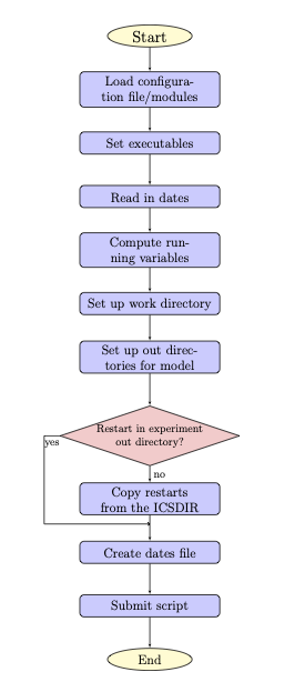
Fig. 6.1 Flowchart of ‘do_submit_cycle.sh’

First, do_submit_cycle.sh reads in a configuration file for the cycle settings. This file contains the information required to run the cycle: the experiment name, start date, end date, the paths of the working directory (i.e., workdir) and output directories, the length of each forecast, atmospheric forcing data, the Finite-Volume Cubed-Sphere Dynamical Core (FV3) resolution and its paths, the number of cycles per job, the directory with initial conditions, a namelist file for running Land DA, and different DA options. Then, the required modules are loaded, and some executables are set for running the cycle. The restart frequency and running day/hours are computed from the inputs, and directories are created for running DA and saving the DA outputs. If restart files are not in the experiment output directory, the script will try to copy the restart files from the ICSDIR directory, which should contain initial conditions files if restart files are not available. Finally, the script creates the dates file (analdates.sh) and submits the submit_cycle.sh script, which is described in detail in the next section.

6.3.2. submit_cycle.sh

The submit_cycle.sh script first exports the required paths and loads the required modules. Then, it reads the dates file and runs through all the steps for submitting a cycle if the count of dates is less than the number of cycles per job (see Figure 6.2).

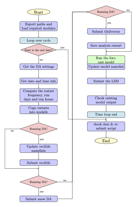
Fig. 6.2 Flowchart of ‘submit_cycle.sh’

As the script loops through the steps in the process for each cycle, it reads in the DA settings and selects a run type — either DA or openloop (which skips DA). Required DA settings include: DA algorithm choice, directory paths for JEDI, Land_DA (where the do_landDA.sh script is located), JEDI’s input observation options, DA window length, options for constructing yaml files, etc.

Next, the system designates work and output directories and copies restart files into the working directory. If the DA option is selected, the script calls the vector2tile function and tries to convert the format of the Noah-MP model in vector space to the JEDI tile format used in FV3 cubed-sphere space. After the vector2tile is done, the script calls the data assimilation job script (do_landDA.sh) and runs this script. Then, the tile2vector function is called and converts the JEDI output tiles back to vector format. The converted vector outputs are saved, and the forecast model is run. Then, the script checks the existing model outputs. Finally, if the current date is less than the end date, this same procedure will be processed for the next cycle.

Note

The v1.0.0 release of Land DA does not support ensemble runs. Thus, the first ensemble member (mem000) is the only ensemble member.

Here is an example of configuration settings file, settings_cycle, for the submit_cycle script:

export exp_name=DA_IMS_test
STARTDATE=2016010118
ENDDATE=2016010318

export WORKDIR=/*/*/
export OUTDIR=/*/*/

############################

# for LETKF,
export ensemble_size=1

export FCSTHR=24

export atmos_forc=gdas

#FV3 resolution
export RES=96
export TPATH="/*/*/"
export TSTUB="oro_C96.mx100"

# number of cycles
export cycles_per_job=1

# directory with initial conditions
export ICSDIR=/*/*/

# namelist for do_landDA.sh
export DA_config="settings_DA_test"

# if want different DA at different times, list here.
export DA_config00=${DA_config}
export DA_config06=${DA_config}
export DA_config12=${DA_config}
export DA_config18=${DA_config}

6.3.2.1. Parameters for submit_cycle.sh

exp_name

Specifies the name of experiment.

STARTDATE

Specifies the experiment start date. The form is YYYYMMDDHH, where YYYY is a 4-digit year, MM is a valid 2-digit month, DD is a valid 2-digit day, and HH is a valid 2-digit hour.

ENDDATE

Specifies the experiment end date. The form is YYYYMMDDHH, where YYYY is a 4-digit year, MM is a valid 2-digit month, DD is a valid 2-digit day, and HH is a valid 2-digit hour.

WORKDIR

Specifies the path to a temporary directory from which the experiment is run.

OUTDIR

Specifies the path to a directory where experiment output is saved.

ensemble_size

Specifies the size of the ensemble (i.e., number of ensemble members). Use 1 for non-ensemble runs.

FCSTHR

Specifies the length of each forecast in hours.

atmos_forc

Specifies the name of the atmospheric forcing data. Valid values include: gdas | era5

RES

Specifies the resolution of FV3. Valid values: C96

Note

Other resolutions are possible but not supported for this release.

TPATH

Specifies the path to the directory containing the orography files.

TSTUB

Specifies the file stub/name for orography files in TPATH. This file stub is named oro_C${RES} for atmosphere-only orography files and oro_C{RES}.mx100 for atmosphere and ocean orography files.

cycles_per_job

Specifies the number of cycles to submit in a single job.

ICSDIR

Specifies the path to a directory containing initial conditions data.

DA_config

Configuration setting file for do_landDA.sh. Set DA_config to openloop to skip data assimilation (and prevent a call do_landDA.sh).

DA_configXX

Configuration setting file for do_landDA.sh at XX hr. If users want to perform DA experiment at different times, list these in the configuration setting file. Set to openloop to skip data assimilation (and prevent a call do_landDA.sh).

6.3.3. do_landDA.sh

The do_landDA.sh runs the data assimilation job inside the sumbit_cycle.sh script. Currently, the only DA option is the snow Local Ensemble Transform Kalman Filter-Optimal Interpolation (LETKF-OI, Frolov et al. [FJSWD22], 2022). Figure 6.3 describes the workflow of this script.

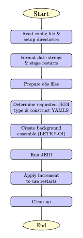
Fig. 6.3 Flowchart of ‘do_landDA.sh’

First, to run the DA job, do_landDA.sh reads in the configuration file and sets up the directories. The date strings are formatted for the current date and previous date. For each tile, restarts are staged to apply the JEDI update. In this stage, all files will get directly updated. Then, the observation files are read and prepared for this job. Once the JEDI type is determined, yaml files are constructed. Note that if the user specifies a yaml file, the script uses that one. Otherwise, the script builds the yaml files. For LETKF-OI, a pseudo-ensemble is created by running the python script (letkf_create_ens.py). Once the ensemble is created, the script runs JEDI and applies increment to UFS restarts.

Below, users can find an example of a configuration settings file, settings_DA, for the do_landDA.sh script:

LANDDADIR=${CYCLEDIR}/DA_update/

############################
# DA options

OBS_TYPES=("GHCN")
JEDI_TYPES=("DA")

WINLEN=24

# YAMLS
YAML_DA=construct

# JEDI DIRECTORIES
JEDI_EXECDIR=
fv3bundle_vn=20230106_public

LANDDADIR

Specifies the path to the do_landDA.sh script.

OBS_TYPES

Specifies the observation type. Format is “Obs1” “Obs2”. Currently, only GHCN observation data is available.

JEDI_TYPES

Specifies the JEDI call type for each observation type above. Format is “type1” “type2”. Valid values: DA | HOFX

Value	Description
DA	Data assimilation
HOFX	A generic application for running the model forecast (or reading forecasts from file) and computing H(x)

WINLEN

Specifies the DA window length. It is generally the same as the FCSTLEN.

YAML_DA

Specifies whether to construct the yaml name based on requested observation types and their availabilities. Valid values: construct | desired YAML name

Value	Description
construct	Enable constructing the YAML
desired YAML name	Will not test for availability of observations

JEDI_EXECDIR

Specifies the JEDI FV3 build directory. If using different JEDI version, users will need to edit the yaml files with the desired directory path.

fv3bundle_vn

Specifies the date for JEDI fv3-bundle checkout (used to select correct yaml).